In this post, I want to explain how to take a normal map and generate its corresponding height map (also called displacement map). There are multiple ways to achieve this, but the one I’ll be covering in this post is the method that Danny Chan presented in Advances in Real Time Rendering at Siggraph 2018 (link here, page 16). It’s also the same method that the Call of Duty engine still uses today to generate the vast majority of its height maps. All the code I’ll cover in this post is implemented here.
Why
There are several reasons why having this process can be helpful:
- The simplest one: very often no height map is available. Even if you aren’t going to actually displace the surface, height maps are useful for a number of reasons, such as blending, or generating quality AO as described in Danny’s presentation linked above (pages 16-22).
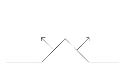
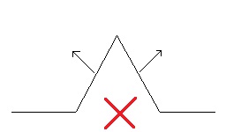
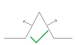
- Even if there is a height map, it’s often ‘wrong’. What I mean, is that the slopes of the surface implied by the height map often don’t match the slopes in the normal map. A height map and normal map are just two different ways of representing the exact same surface, and they are intrinsically linked together. For example, say you’re displacing the ground, and it creates a small 45-degree hill. If your normal map returns a slope of 80 degrees, then you’ll be lighting the hill as if it should be steeper, and it will just look off:
The majority of painted or edited height maps just won’t have this guarantee of matching the normals (or vice versa), and therefore be wrong. While the above image could just have either the heights or normals scaled to fix the mismatch, it’s also common with painted normal maps where they end up being ‘impossible’ (there exists no surface that could match the slopes). In general, normal maps that are captured through photogrammetry are the best ones. However, even if you’re using photogrammetry assets, the height map provided with them is often cleaned up or scaled to look ‘pretty good’, but not actually made to match the normal map very well (I’ll show an example of this later).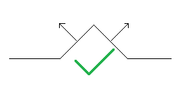
- Nearly all engines provide two extra parameters when doing displacement: displacement scale and bias. In most of those, changing the displacement scale causes the geometric and normal slopes get out of sync.
This is because usually the displacement height and normals are calculated completely independently from each other in the shader:
displacementHeight = scale * sampledHeightMapValue + bias;
displacedNormal = regularNormalMappedNormal;
Really though, changing the displacement scale changes the slope of the geometry, so the normal should be scaled as well. You can play around with the displacement bias as much as you want since that just moves the whole surface, but changes to the scale mean the normals need to be scaled as well. The reverse is true as well: scaling the normals means you need to change the height map or displacement scale too.
Because of reasons #2 and #3 above, the Call of Duty pipeline actually doesn’t allow you to use a hand-authored height map and a normal map at the same time on a material. You can either:
- Provide only a normal map and have the height map auto-generated from the normal map using the method I’ll describe in the rest of this article.
- Provide only a height map and have the normal map auto-generated from the height map.
In both cases, it ensures that the height map and normals will always match. A follow-up question is then “what about the displacement scale”? The scale is no longer tied to the material, but the textures themselves:
- If using a normal map, a new float parameter is introduced to scale the normals. The normals will be scaled before generating the height map.
- If using a height map, then you can simply scale the heights before generating the normal map.
In both cases again, the maps will be matching. Now that that’s all explained, let’s dive into how this normal-to-height generation actually works.
How it works
Core Idea
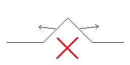
The algorithm itself is actually pretty short. The core idea is that for any pixel, we can estimate its height given the heights and slopes of its neighbors. Take the image below for example, where we want to estimate the height of the center pixel '?'.
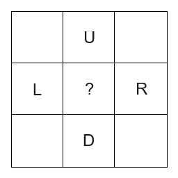
L + Slope(L).x. Another guess would be D - Slope(D).y (note that we are assuming that normals the normals are +Y down, and +X to the right, but you can flip the signs if your normal maps are different). We can do this for all 4 neighbors, and take the average to get a pretty good guess for the middle’s height.
You might be confused though, “we don’t know the neighbor’s heights yet”? Correct, but it doesn’t matter! The cool thing about this algorithm is that if you just make an initial guess for the heights, and do this neighbor guess averaging over and over, it will eventually converge! So if we start with a guess of all heights = 0 and iterate a bunch of times, it converges to the final height map we want. Pretty neat, right? There are some other details and tricks to speed up the convergence though, so let’s get into the specifics.
Implementation
So the first part of the algorithm is to convert the normals into slope space. This is just the partial derivatives of the height field with respect to X and Y. Aka, how much the height changes in the X and Y directions:
\[ \frac{\partial z}{\partial x} = \frac{-n.x}{n.z} \] \[ \frac{\partial z}{\partial y} = \frac{-n.y}{n.z} \]vec2 DxDyFromNormal( vec3 normal )
{
vec2 dxdy = vec2( 0.0f );
if ( normal.z >= 0.001f )
dxdy = vec2( -normal.x / normal.z, -normal.y / normal.z );
return dxdy;
}
We do this for every pixel in the normal map and divide by the input texture size. This is just to normalize the slopes to be independent of the texture size. Without it, the height map would get taller as you increased the normal map size for example.
FloatImage2D dxdyImg = FloatImage2D( width, height, 2 );
const vec2 invSize = { 1.0f / width, 1.0f / height };
for ( int i = 0; i < width * height; ++i )
{
    vec3 normal = normalMap.Get( i );
    dxdyImg.Set( i, DxDyFromNormal( normal ) * invSize );
}
The last thing to do before we get to the meat of the algorithm is to allocate two more images: the final output height map (last argument), and a scratch height map. The latter is just used internally by the algorithm during iteration, which we will see in a second.
FloatImage2D scratchHeights = FloatImage2D( width, height, 1 );
FloatImage2D outputHeights = FloatImage2D( width, height, 1 );
BuildDisplacement( dxdyImg, scratchHeights.data.get(), finalHeights.data.get() );
Now the core of BuildDisplacement is the repeated averaging of the height guesses I explained earlier. This iteration method is also called relaxation. You could do this on the current resolution as-is, but it would take a long time to converge (often tens of thousands, or hundreds of thousands of iterations). As the presentation mentions, to speed up the convergence you can instead: recursively downsample the image, iterate on that a smaller number of times (tens, or hundreds of times, not thousands), and then upsample that to use as the starting guess for next round of iterations. Confusing? Here’s the code:
void BuildDisplacement( const FloatImage2D& dxdyImg, float* scratchH, float* outputH )
{
    int width = dxdyImg.width;
    int height = dxdyImg.height;
    if ( width == 1 || height == 1 )
    {
        memset( outputH, 0, width * height * sizeof( float ) );
		return;
    }
    else
    {
        int halfW = Max( width / 2, 1 );
        int halfH = Max( height / 2, 1 );
        FloatImage2D halfDxDyImg = dxdyImg.Resize( halfW, halfH );

        float scaleX = width / static_cast<float>( halfW );
        float scaleY = height / static_cast<float>( halfH );
		vec2 scales = vec2( scaleX, scaleY );
        for ( int i = 0; i < halfW * halfH; ++i )
			halfDxDyImg.Set( i, scales * halfDxDyImg.Get( i ) );

        BuildDisplacement( halfDxDyImg, scratchH, outputH );

		// upsample the lower resolution height map, outputH, into scratchH
        stbir_resize_float_generic( outputH, halfW, halfH, 0,
			scratchH, width, height, 0, 1, -1, 0, STBIR_EDGE_WRAP,
			STBIR_FILTER_BOX, STBIR_COLORSPACE_LINEAR, NULL );
    }

	... neighbor iteration ...
Let’s walk through an example image of size 32x32. It would first downsample the slope image to 16x16: halfDxDyImg = dxdyImg.Resize( 16, 16 ). The next step is to update the slopes to account for the bigger pixel footprint. Remember we initially divided the slopes by the texture size: DxDyFromNormal( normal ) * invSize. So each slope in that image was describing “how much does the height change if we move 1/32nd of a unit”. Each texel in the lower resolution image now describes “how much does the height change if we move 1/16th of a unit”, so we need to double the slopes from the higher resolution image.
Next, we call BuildDisplacement again until we get down to a 1x1 image. Here we seed the initial guess of all heights to 0. You can use something other than 0, the only thing it changes is where the average height of the final image is (moves the entire surface up/down). It will then upsample to 2x2 and do the neighbor iteration. Then upsample that to 4x4 and do the neighbor iteration again, then 8x8, etc. So how does the neighbor iteration look exactly?
float* cur = scratchH;
float* next = outputH;
// ensure numIterations is odd, so the final output is stored in 'next' aka outputH
numIterations += numIterations % 2;

for ( uint32_t iter = 0; iter < numIterations; ++iter )
{
    #pragma omp parallel for
    for ( int row = 0; row < height; ++row )
    {
        int up = Wrap( row - 1, height );
        int down = Wrap( row + 1, height );

        for ( int col = 0; col < width; ++col )
        {
            int left = Wrap( col - 1, width );
            int right = Wrap( col + 1, width );

            float h = 0;
            h += cur[left  + row  * width]  + 0.5f * dxdyImg.Get( row, left ).x;
            h += cur[right + row  * width]  - 0.5f * dxdyImg.Get( row, right ).x;
            h += cur[col   + up   * width]  + 0.5f * dxdyImg.Get( up, col ).y;
            h += cur[col   + down * width]  - 0.5f * dxdyImg.Get( down, col ).y;

            next[col + row * width] = h / 4;
        }
    }
    std::swap( cur, next );
}
A few notes on this:
- The neighbor averaging can’t be done in place (much like a blur filter), which is why it flips between scratchH and outputH each iteration. The code is written to assume that the final iteration will store into outputH, which means we must have an odd number of iterations (store results in outputH on iteration 1, scratchH on iteration 2, outputH on iteration 3, etc.).
- You can also see that I just made the assumption that all of these input textures wrap. If they can’t wrap, then you can try the usual tricks at the edges (clamp/reflect). To be honest, I haven’t tried it yet personally.
- All of the slopes are multiplied by 0.5. Embarrassingly, I have no idea why this is needed! I found out it gives much better results accidentally when I was trying to average the neighbor slopes with the center pixel’s slope (the center slopes cancel out anyways, but the 0.5 multiplier significantly improved things). Perhaps I missed a factor of 2 somewhere else, not sure.
After that, the only remaining step is to remap the final image to be 0 - 1, for minimal loss when saving it out (if saving the result out as 8 or 16-bit). The scale needed for remapping (maxHeight - minHeight) is the same needed later in the shader for unpacking. The same goes for the bias (minHeight).
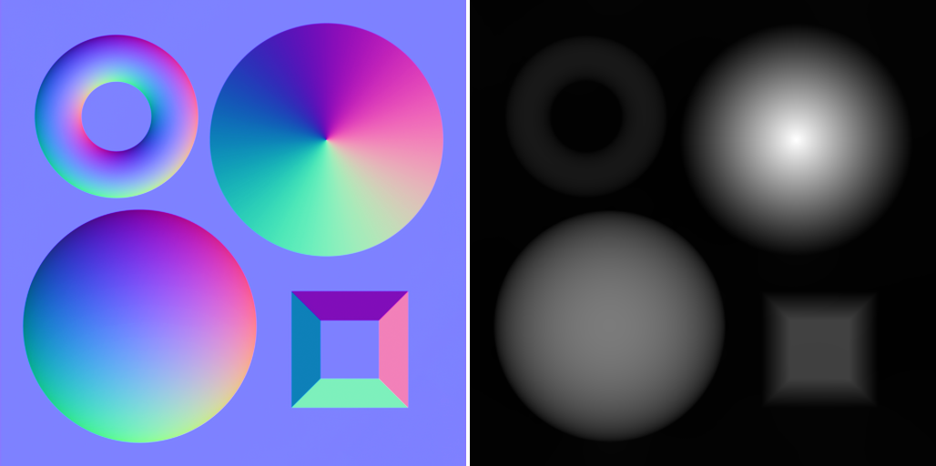
The Results
It’s a bit of a challenge to quantify exactly how good the generated height maps are, particularly when we don’t have ground truth images to compare them to! The only ground truth images we have are the normal maps. Because of that, I took the generated height maps and generated normal maps from those. That way we can do direct comparisons and gather standard image diff metrics (MSE/PSNR). Now, there is a huge caveat here: both the normal-to-height and the height-to-normal processes introduce error. So by comparing the two normal maps, we are actually measuring the combined error of both processes, not just the first normal-to-height error that we would like. But it’s better than nothing, so here we go.
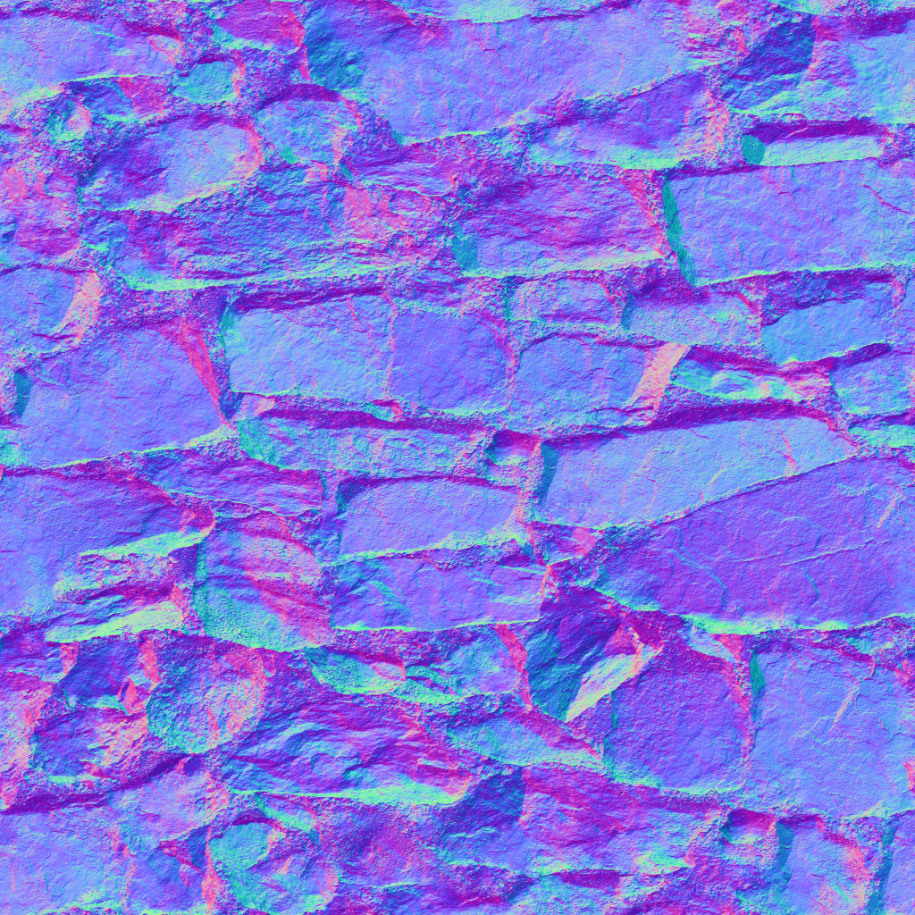
Below are the results of 5 test cases (3 photogrammetry, 2 synthetic). The first column is the starting ground truth normal map, the second column is the generated normal map, and the third column is the generated height map. There are many ways to generate normals from a height field, I chose the simplest one for this, just doing the finite difference between the left + right neighbors, and the up + down neighbors (search for GetNormalMapFromHeightMap in the code). All of these height maps were generated using 1024 iterations. To get the PSNR between the two normal maps, I generated the dot product between both images, adjusted so that 0 means both vectors are the same, and 2 would mean they are completely 180 from each other: 1 - Dot( n1, n2 ). I then found the MSE of that dot product image and converted that to PSNR (search for CompareNormalMaps in the code). Here were the results (click images to enhance and flip between them):
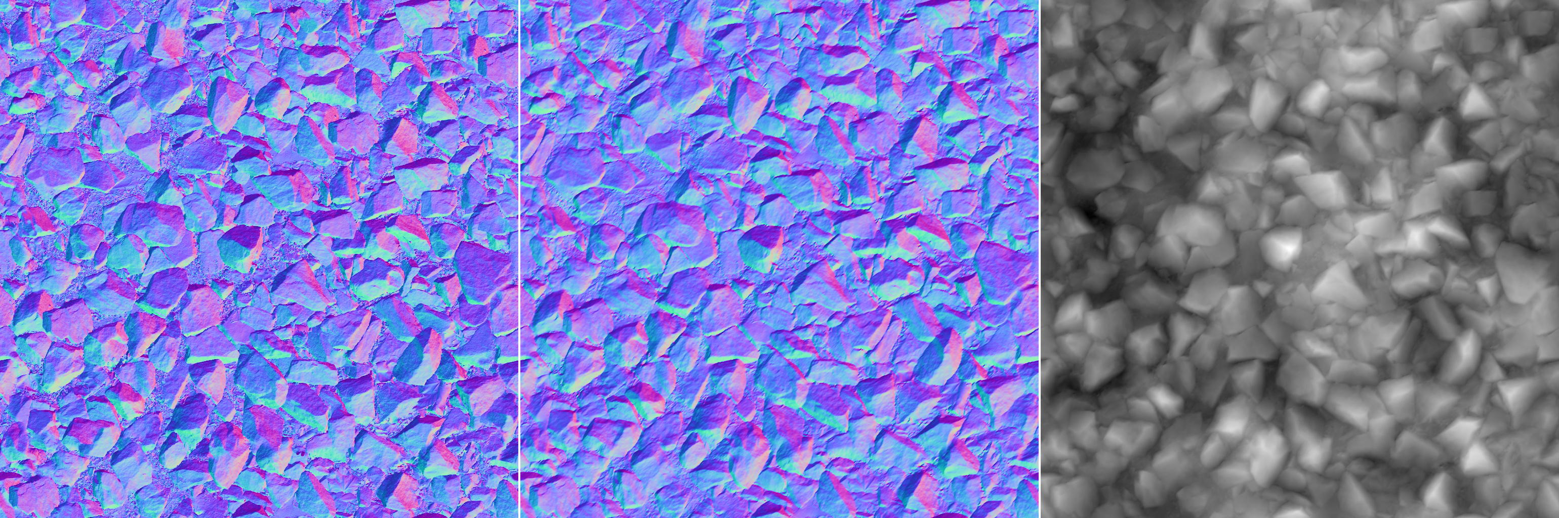
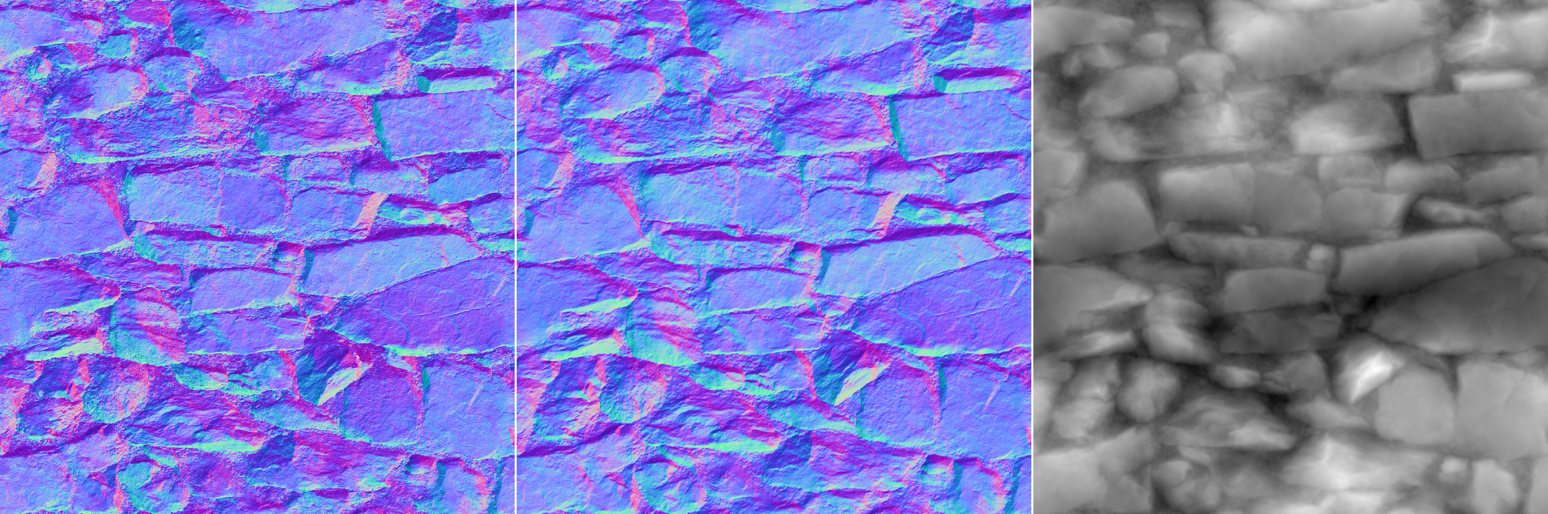
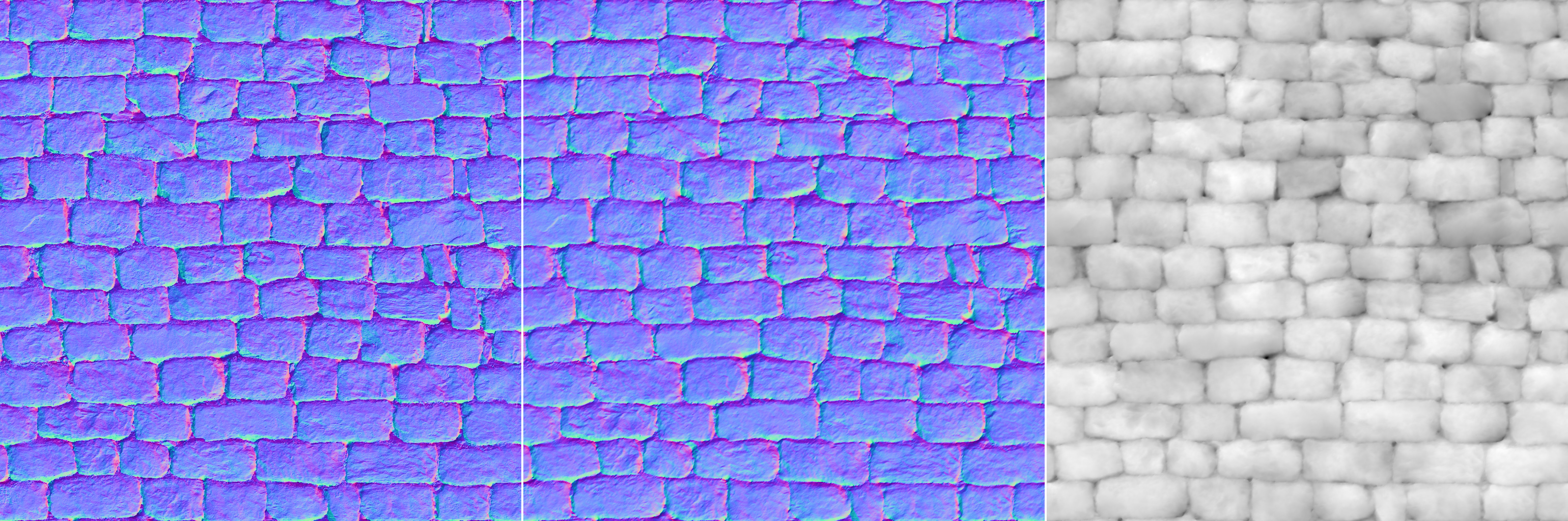
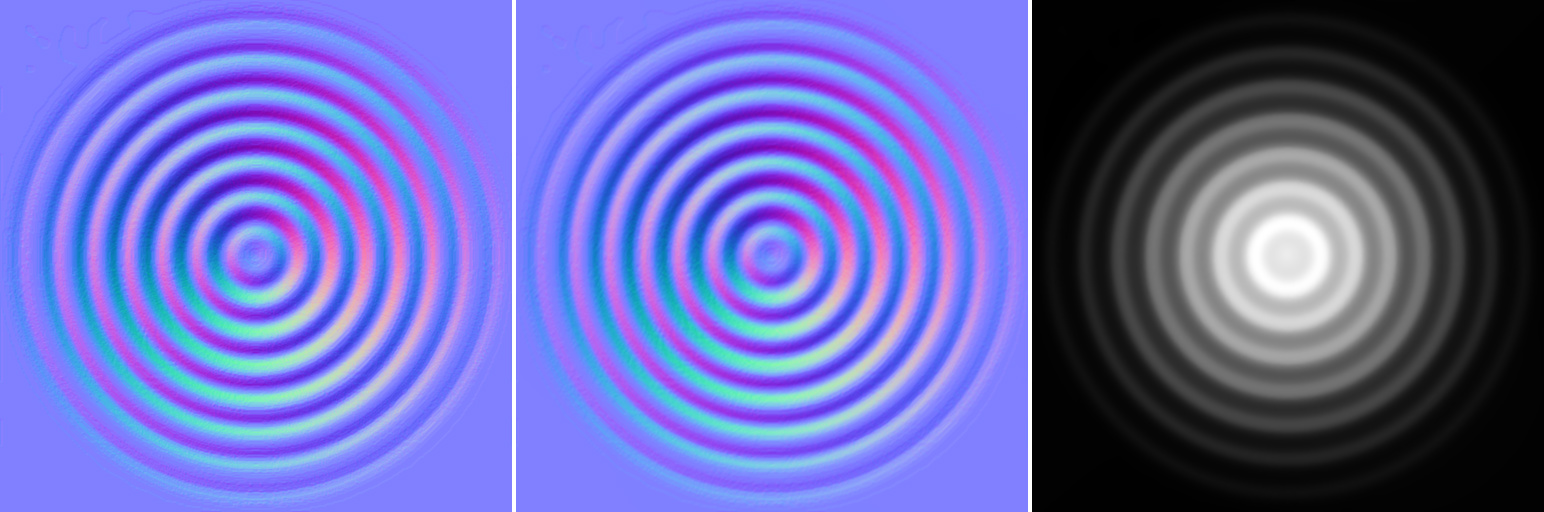
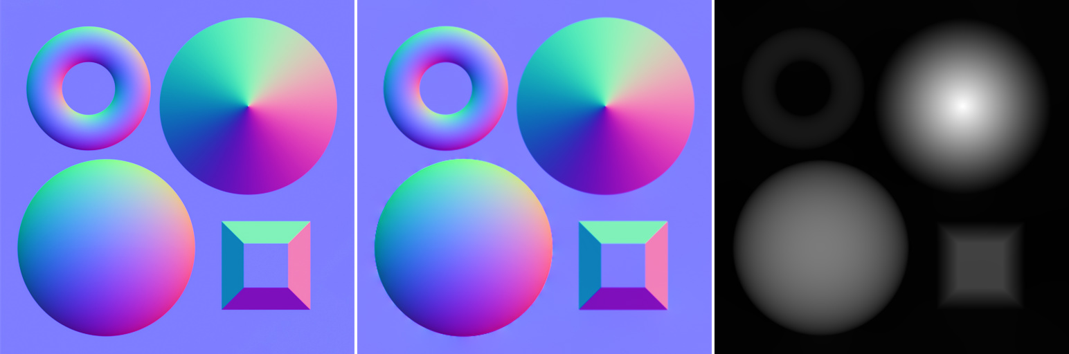
Pretty good in my opinion! If you really squint, you can see where it doesn’t do so well. The last synthetic image is a nice example of how it doesn’t do well at sharp corners. Some of that is just due to the error in the height-to-normal process, but some of it also is from the height generation.
Compared To Provided Height Map
Remember when I said that sometimes even with photogrammetry, the provided height map just doesn’t match the normals that well? The 2nd rock image above is a good example of this.
This asset is from Poly Haven, which is wonderful and actually provides a blender file that lets us see what the author says the scale should be. In this case, it’s 0.20. However, look what happens when we generate the corresponding normal map, using the provided height map + 0.20 scale:
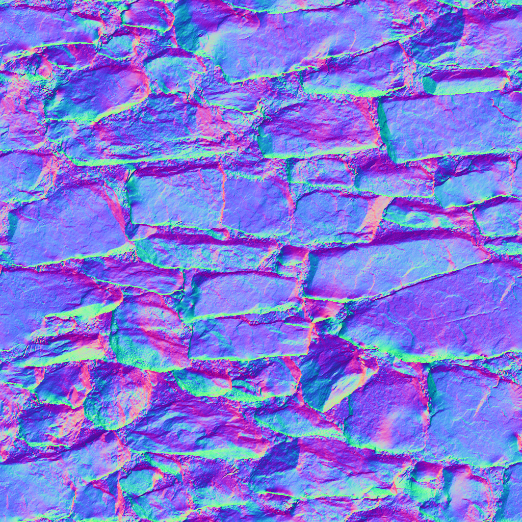
It basically kept all of the flatter top surfaces accurate, but heavily increases all the other slopes. It also has a PSNR of 20.6. If we get rid of the 0.20 scale and do a search for the scale that makes for the best PSNR, we find that a scale of 0.065 gives us a PSNR of 23.5:
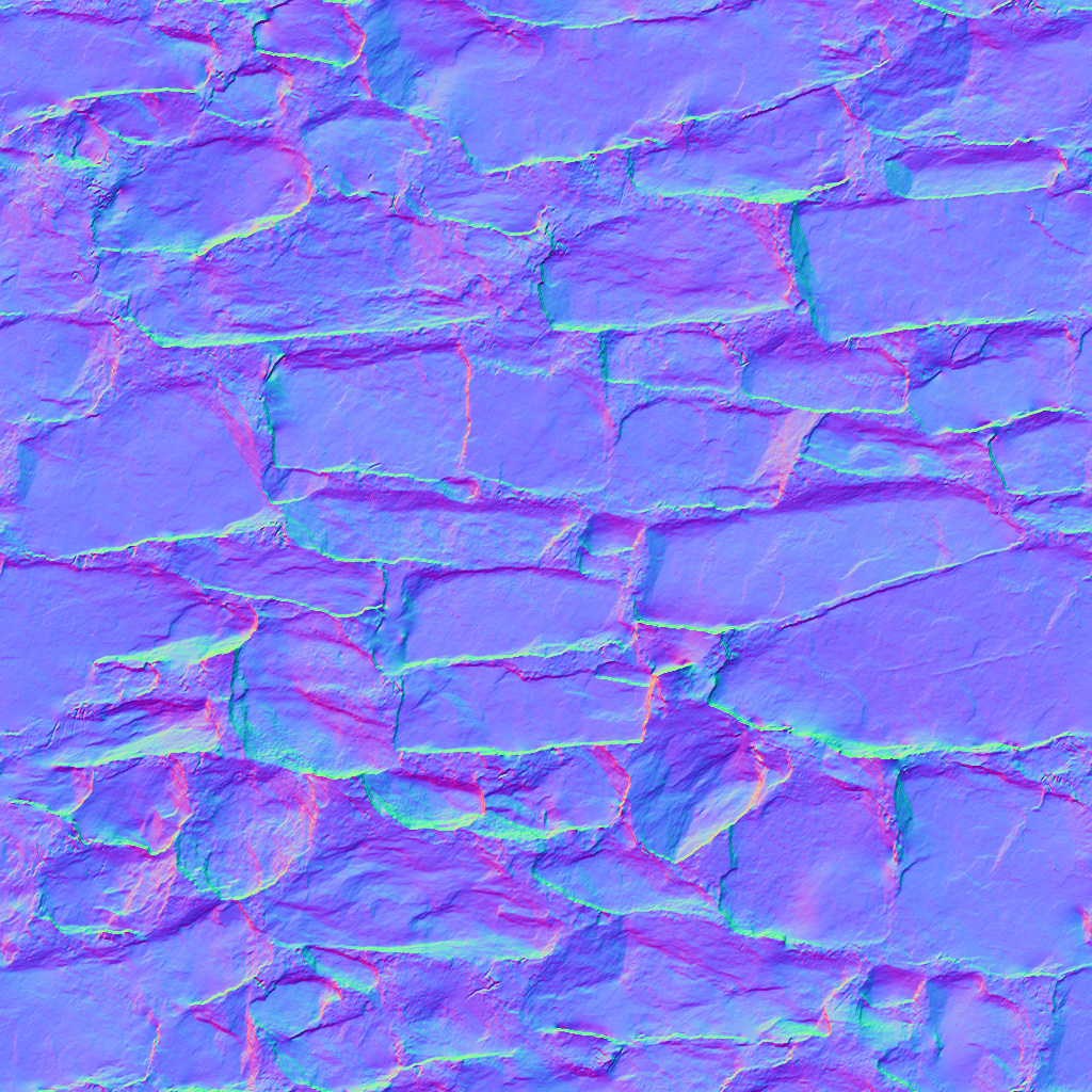
Now we have the opposite problem: the steeper slopes and crevices were preserved better at the cost of flattening everything else. This means that really, there is no scale that will preserve both areas– the map itself just doesn’t match the normals well. If we use the auto-generated height map, however, you can see that it matches a lot better. Not perfectly, but definitely more than the provided height map can:
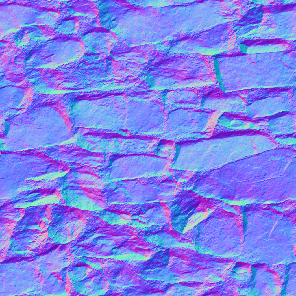
For the record, I’m not blaming the author of this material at all. This is a great asset to have, and I bet it still looks pretty good when displaced. But if your goal is to have the geometric and normal slopes match like we have been arguing it should, then the height map isn’t quite the best for it. So just a warning that just because a material was captured with photogrammetry doesn’t mean it’s always perfect.
How Long To Iterate?
You might notice that I didn’t define numIterations anywhere in the code snippets above. I was glossing over that because it’s a bit trickier to answer! The longer you run this algorithm, the longer it has to converge. How do you know when it is done converging? There are a couple of ways you could define convergence and measure it. Since our initial guess was a flat surface, however, a pretty good way you can tell if it has converged is when the surface stops getting taller as you increase the number of iterations. Even for images with lots of crevices and details in the middle height ranges, tracking the total height still seems to be a good way of defining total convergence, at least with all of my test cases. Now, you can track the min and max height after each iteration to do this, but:
- The height changes are very small per iteration and get increasingly smaller with each further iteration. That means you’ve really just swapped to a new, equally hard problem: what should the super small threshold be exactly?
- It’s slightly more annoying and slower to track each iteration since we are multi-threading.
The option I took instead was to just try a bunch of different iteration counts on a number of images and see how they converged. Below is the results of 7 different normal maps, where the height map was generated at 9 different iteration counts: 32, 64, 128, 256, 512, 1k, 2k, 4k, and 32k. If we consider the scale given by the 32k image as ‘fully converged’ we can then divide all of the other scales (per image) by that to normalize everything:

You can see that there is some slight variation between normal maps, but they all pretty closely follow the same trend. Basically everything above 2k is imperceptible, and 512-1024 iterations are probably more than enough for the vast majority of images. I default to 512 as being ‘good enough’, but you can pick whatever iteration count you feel is most appropriate for your application. For many applications, sub-100 iteration counts can be perfectly fine. I will say that if you are using these as displacement maps though, I have noticed iteration counts under 100 can sometimes (not always) be noticeably not done converging, like where sections of geometry that should be straight are actually curved because it didn’t converge yet.
Can We Make The Algorithm Faster?
There are a few obvious ways this code could be improved: the parallelization could be better, the downscaling of the dxdy image and upscaling of the height image could for sure be sped up (I was just using the easiest stb option for them), and you could likely do more intelligent ways of calculating numIterations. Implementing those isn’t the point of this post though, the question I want to ask here is: can the algorithm itself be tweaked to be faster? Turns out, the answer is yes!
Take one of the rock textures from above, which has size 1024x1024. If we save out all of the intermediate height maps (what BuildDisplacement returns) and scale them up to 1024x1024 for comparison, we get the following (sizes 8x8 to 1024x1024):


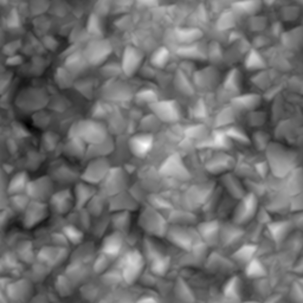


You can see that pattern: as the mips get larger, the less impact each set of iterations has. This makes sense– you would hope that once all of the iterations on the 1x1 -> 128x128 sized mips are done that all of the details sized >= 1/128th of the image would be done converging. So, there should be less work to do as the image gets larger, because the larger iterations have better and better initial guesses and will mostly just be converging the smaller and less noticeable details.
So what if we reduced how many iterations just the largest mips got? To do this, let’s introduce an iteration multiplier. It will scale the number of iterations of mip 0 by that amount, and then we can double the multiplier for the next mip. This way we have fewer iterations on the larger mips, but the same amount on the smaller ones:
void BuildDisplacement( const FloatImage2D& dxdyImg, float* scratchH,
	float* outputH, uint32_t numIterations, float iterationMultiplier )
{
	...

	BuildDisplacement( halfDxDyImg, scratchH, outputH,
		numIterations, 2 * iterationMultiplier );

	...

	numIterations = (uint32_t)(Min( 1.0f, iterationMultiplier ) * numIterations);
	numIterations += numIterations % 2; // ensure odd number
	...
The results? If we do 1024 iterations with a 0.25 multiplier on the rocky image above, we get nearly the exact same quality as a 512 iteration with a 1.0 multiplier, but 25% faster. What if the image was larger though? We are predicting that those details matter less and less. It turns out the prediction is true! Doing 1024 iterations with a 0.25 multiplier on a 2048 version of this same image gives the same quality as doing 710 iterations, but again faster than 512. If we do the same with a 4096 version of the image, it gets even better: the same quality as doing 794 iterations, but the same cost as doing 350 iterations!
So what multiplier should you use? Like the number of iterations, it just depends on what quality you want and how fast you want it. Remember this also works better on larger images like 2k or 4k. I like to default to 1024 iterations with 0.25 multiplier, especially with 1k+ images, but adjust it as you see fit!
Future Work
While this method works well (don’t forget it’s used in AAA games like Call of Duty!), there are a lot of questions and issues we ignored:
- Since the height algorithm always pulls from its neighbors, it’s guaranteed to mess up (smooth) sharp corners
- Similarly, the way we reconstructed the normals increases how much error there is at sharp corners, making it harder to examine the error from each step
- Explaining why as you increase the iteration count, the PSNR almost always goes down slightly
- If you zoom in and compare the original and generated normal maps, you’ll notice the generated one has most of the high frequency details blurred out
- Are there alternative ways to generate the height maps that might be better or faster?
And more. I think this post is definitely long enough as-is, however, so I’m going to write a part 2 where I dig deeper into these issues and try to answer some of these questions. Once that is posted, I’ll update this page with a link to it.
Credits
Huge thanks to the providers of the source normal maps (list of each one, and links to them can be found here).